This blog post is part of a series on using large language models for text classification. View the other posts here:
-
LLMs for Text Classification: A Guide to Supervised Learning
-
Text Classification With LLMs: A Roundup of the Best Methods
By Benjamin Nativi, Will Porteous, and Linnea Wolniewicz
The rise of large language models (LLMs) has spurred feverish excitement about the capabilities of AI. But the ability to generate useful text and images on demand has overshadowed how to use LLMs for traditional machine learning tasks, such as text classification.
Our first post in this series on text classification using LLMs focused on supervised learning. It detailed how approaches like fine-tuning existing frameworks and using a classification head with a pre-trained model can work to sort text into categories.
But supervised learning is only one trick up a data scientist’s sleeve. In this post, we explore unsupervised text classification—a fundamentally different approach to machine learning.
Can a machine learning model succeed at classifying text without labeled data?
Can it do the job as well as a model that has labeled data?
Which approach gives the best results for the least amount of computational resources?
Let’s find out.
What Is Unsupervised Text Classification?
First, let’s clarify unsupervised learning. Unsupervised learning is one of the main areas of machine learning. While supervised learning uses labeled input data (typically labeled by a human) to train models, unsupervised learning uses no (or very few) labeled data points. However, in our case, unsupervised learning uses a pre-trained model to perform a new task that it wasn’t trained to do without updating the model.
For our experiments with supervised learning, we fine-tuned common text classification models on a standard natural language processing (NLP) dataset, the Text REtrieval Conference (TREC) Question Classification dataset. We also used another method, which involved applying a classification head to a pre-trained Llama model to take advantage of transfer learning. All of these approaches involved training models.
Our unsupervised text classification experiments did not train any models. Instead, they centered on prompt engineering—a process of instructing an LLM to classify inputs based on constructed prompts rather than fine-tuning any models themselves. We evaluated these models on AG News, a dataset of news articles that fall into four categories: world, sports, business, and technology.
How Can We Use Unsupervised Learning With LLMs for Text Classification?
Since LLMs have such strong general language capabilities, it is reasonable to assume that they may be able to perform text classification tasks. Yet, even the most advanced LLMs of the current generation cannot interpret text without proper instructions. After all, they are trained to generate text, not label it. If an LLM simply receives a line of text, it will continue it rather than classify it.
Instead, there are two main strategies for encouraging an LLM to classify text:
- Provide the LLM with instructions.
- Provide the LLM with labeled examples.
For example, an instructive prompt could be: “Classify the news article as world, sports, business, or technology news.” Likewise, a labeled example could be “Article: Striveworks secures patent for innovative data lineage process. Class: Technology.”
In both cases, the instructions or examples must be included in the textual input to the LLM as LLMs are not designed with special inputs for instructions or examples. The instructions or examples must be integrated with the query (the text that the LLM should classify) to form one string of text.
Important Considerations for Constructing Prompts
In our experiments, we first tried to provide instructions without examples. This is known as zero-shot prompting because zero is the number of examples—or “shots”—provided. This method does offer computational advantages over alternatives, but its biggest advantage is that this method requires no labeled data. Once the data is cleaned and properly formatted, the only additional work required is to write the instruction.
There are a few important considerations when drafting instructions for LLMs. Most importantly, prompt engineers must recognize that the performance of an LLM on a task can vary significantly based on small changes to the phrasing of the instruction. For example, the authors of the Llama LLM say that users should refrain from asking questions such as, “Is this news article an example of world, sports, business, or technology news?”
Llama was not trained to answer questions, so the text it generates in response may not be a valid answer. Instead, Llama responds much better to commands such as, “Classify the news article as world, sports, business, or technology news.”
Instructions can be even more important for other LLMs, such as Alpaca, which were fine-tuned specifically for instruction answering.
It is also helpful for prompt engineers to clearly identify the location of the input and the location of the output in their prompts. For example:
Classify the news article as world, sports, business, or technology news.
Article: Striveworks secures patent for innovative data lineage process
Class:
By formatting the text in this way, the LLM is provided an instruction, and the news article is clearly identified. Ending with the text “Class:” indicates to the model that the text it outputs should be the class of the news article. Because the possible labels were provided in the instruction, the LLM is encouraged to use those same labels to classify the article.
To get the class suggested by the model, one possible method is to look at the model’s response to the prompt. LLMs respond by generating a new token (i.e., a word or part of a word). Then, we can look at the token and see which label it matches. This may be effective, but it can create issues. Smaller models like Llama sometimes generate outputs that don’t correspond to the labels—even when given instructions. In one case, instead of outputting a class, Llama started a second, fictitious news article: Article: Llama model shows high performance despite smaller size. Even bulky models such as GPT, with over a trillion parameters, occasionally mess up. GPT sometimes produces labels that do not exactly match the true labels (producing “legal” instead of “technology” for the above article).
Instead of letting the model generate a new token, we can analyze the probabilities that each of the true labels (world, sports, business, technology) will be produced and then take the label with the highest probability. A similar effect can be achieved by restricting the LLM to only output the true label tokens. These are more reliable and higher quality methods for using LLMs to classify text than by simply taking their output at face value.
In Figure 1, we show the results of our evaluation of five different LLMs with zero-shot prompting. Each model was evaluated on the same 1,200-point test set with the same prompts.
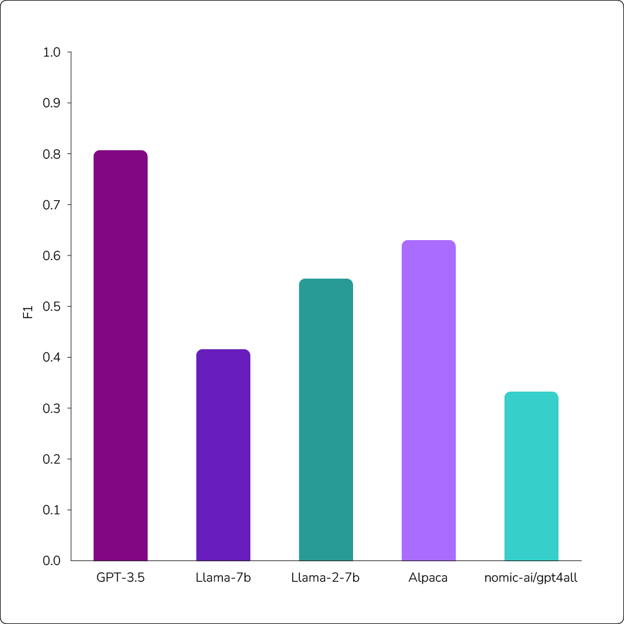
Figure 1: Results of zero-shot prompting experiments using GPT-3.5, Llama-7b, Llama-2-7b, Alpaca, and gpt4all large language models. While GPT-3.5 returned the most accurate results, all models underperformed when compared with supervised learning models.
On this dataset, most of the F1 scores are quite poor. (F1 scores are a measurement of accuracy for model performance.) For reference, the supervised learning model DistilRoBERTa achieves an F1 score of 0.947 on this same dataset with access to the entire 120,000-point training set. Although this is not a fair comparison, we would still want to see results that are much closer to the supervised fine-tuning methods to consider using one of these models with zero-shot prompting.
Both Llama and the recently introduced Llama 2 models achieve some nontrivial performance, but they are still quite poor. Alpaca and Nomic AI’s gpt4all (no relation to OpenAI’s GPT model) are both instruction-tuned, yet gpt4all performs very poorly, and Alpaca is just slightly better than Llama 2. The only model to achieve reasonable performance is GPT 3.5, with an F1 score close to 0.8. While this result is decent and shows that larger LLMs have more potential to be used without any labeled points, it is still far worse than fine-tuning methods.
GPT also presents an issue that the other models do not. Because the other models are open source, we are able to work with the logits directly to assess the probabilities of the models’ output labels and confirm a valid label. For every input, we got a valid label, and we could compute the F1 score from the corresponding confusion matrix. However, GPT is not open source and only returns the text it generates. For this inference run, GPT only provided valid labels on 90% of the queries. To compute an F1 score, we randomly assigned labels to the remaining 10% of queries and computed the F1 score from there. The F1 score for GPT on the 90% of queries with valid labels was actually about 0.88, which is pretty good, but it does not capture the poor performance on 10% of the test set.
k-Shot Prompting
Fortunately, there are alternatives to zero-shot prompting. If we want better performance and we are willing to label a few examples, we can use an approach known as k-shot prompting. Let’s look at how to use this approach and how it affects performance.
Unlike zero-shot prompting, k-shot prompting provides an LLM with examples (aka “shots”) of correct classifications. K is equal to the number of examples provided. Here is an example of a 4-shot prompt using AG News data:
Classify the news article as world, sports, business, or technology news.
Article: Biden addresses G7, emphasizing need for increased unity
Class: world
***
Article: Losing streak extends to seven games for the Boston Bruins after another dismal performance on Tuesday evening
Class: sports
***
Article: Wall Street doubles down on risky investments as leading economists sound the alarms
Class: business
***
Article: Honda is preparing to introduce an improved speech-recognition system in partnership with IBM
Class: technology
***
Article: Striveworks raises $33 million in first institutional round
Class:
Part of the work in k-shot prompting is the same as in zero-shot prompting—writing the instruction. Although it may seem like the instruction is no longer necessary, including the instruction added little computational cost but typically led to small performance gains in our experiments. However, we also found that the specific wording and formatting of the instruction had less impact on the performance when we provided more shots.
Aside from the instruction, k-shot prompting comes with an additional consideration—the shots. In this approach, there are many new questions we can ask:
- Are there clever ways to select which shots to provide?
- Does performance improve if we provide more shots?
- What limitations do we face in providing more shots to the LLM?
Sampling Strategies
Of course, with a collection of unlabeled data points, we could opt to label a few random data points to use as shots. But what if we could select shots that were more helpful than random? Or, what if we labeled more data points and used different examples for different queries? These options divide sampling strategies into two categories: static strategies and dynamic strategies.
With a static sampling strategy, shots are fixed; the same shots are used for every query in the dataset. The most basic strategy here is the random selection mentioned above.
Sampling Through k-Means Clustering
One alternative to random sampling, though, is k-means clustering. With k-means clustering, data points are turned into vectors and embedded into a vector space. For NLP, turning a string of text into a vector involves putting the text through an embedding model, which assigns each token in the string an integer and then applies a mathematical function to those integers to arrive at a vector that represents the meaning of the text. For these experiments, we used a BERT-based embedding, Sentence-BERT, since this embedding has been shown to be useful for this purpose.
Once the data has been vectorized, it gets plotted in the vector space. The distance between data points in this vector space represents the similarity between the data points. Once plotted, the unlabeled data gets clustered into k clusters. For each cluster, the data point closest to the center of the cluster gets labeled and used as a shot. In this way, the k shots are dissimilar from each other, so the shots provided to the LLM are a diverse sample from the dataset. The hope in using this method is that a diverse selection of shots will help the LLM better distinguish between the classes.
Random Resampling Strategy
Conversely, with a dynamic sampling strategy, the shots used in each query may be different. As a baseline, we evaluated a random with resampling strategy, where we just resampled the random shots for each query. We shouldn’t expect an improvement in performance here, but changing the shots between inferences should reduce the variance between runs.
Nearest Neighbors
For a smarter dynamic strategy, we evaluated nearest neighbors. In nearest neighbors, we first embed the labeled points as in k-means clustering (again with a BERT-based embedding). Instead of selecting data points from ranging clusters, though, we select the k closest labeled points in the vector space to use as examples. In a sense, this approach is the opposite of k-means clustering. While that approach aims to select shots that are as diverse as possible, nearest neighbors aims to select shots that are as similar as possible (with the expectation that these shots may be most relevant for the LLM).
Static vs. Dynamic Sampling Strategies: Results
In Figure 2, we show how 23-shot prompting using each sampling strategy performed with Llama on the AG News dataset. We evaluated on the same 600-point subset of the standard test set and did five runs of each strategy, showing the range between the best and worst runs. Each random run used a different set of random shots for the whole run. For k-means, each run is distinct because different subsets of the data are used for each run for clustering, thus getting different examples. For random resample and nearest neighbors, different subsets of the training set were used for each run.
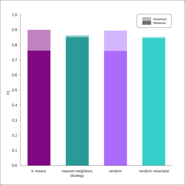
Figure 2: Results of sampling strategies used with 23-shot prompting. Surprisingly, all methods returned similar F1 scores, suggesting that random sampling is sufficient with Llama when incorporating enough shots.
As we can see, all sampling strategies returned roughly the same average F1 score (0.83 to 0.85). The static strategies did have a higher variance between runs, but this matters little—a technique for reducing variance (ensembling, which we discuss later) also has the benefit of improving the average F1. Other than this difference, the similar performance is quite surprising. We expected a thoughtful choice of examples to give better results, but our experiments have shown that random sampling is sufficient with Llama when prompters keep the shot count high. This contrasts with much of the literature on GPT, where others have found improvements from different sampling strategies. We should note that we tried other static and dynamic strategies that are not shown here, but none did any better than what we have shown.
Ultimately, it seems that smaller LLMs like Llama are much more affected by factors other than shot variance, as we will discuss below.
Shot Number
Next, we consider F1 versus shot number. We evaluated our tests on the same 1,200 point subset of the standard test set and did five runs for each shot number (except for zero-shot). For each run, we used a different set of random shots, so it did not make sense to do multiple runs of zero-shot. In Figure 3, we show the minimum and maximum F1 scores for five runs of each shot count to give a sense of performance, as well as variance, between runs.
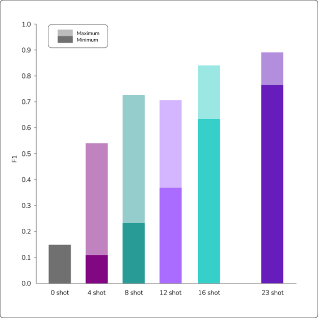
Figure 3: Results of experiments using varying numbers of shots for each prompt. Higher shot counts consistently produced more accurate results in our tests.
As we can see, there is a strong correlation between the number of shots and the F1 score. With smaller shot counts, some runs obtain decent F1 scores, but there is a lot of variance between runs, and the best run of 4-shot, 8-shot, and 12-shot are still worse than the worst run of 23-shot. We can see that as the shot count increases, not only does the average F1 score increase, but the variance between runs also decreases. This information may be useful as it gives us a sense of the minimum performance we can expect. Even for 16-shot, which obtains a decent maximum F1 score of 0.84, the minimum F1 score of 0.63 is pretty bad. With 23-shot, the maximum of 0.89 is not far off fine-tuning methods, and the minimum of 0.76 isn’t terrible.
Ensembling to Overcome LLM Context Limitations
If performance improves strongly with shot count, why stop at 23 shots? The problem is that LLMs have limited context sizes. LLMs have a maximum number of tokens they have been trained to attend to. In the case of Llama, that is 2,048. This means that the token lengths of the instruction, all of the shots, and the query must add up to no more than 2,048 tokens. Combining the length of the instruction and the maximum token length of a query in the test set gives a maximum number of tokens that can be used for shots. Dividing 2,048 by the length of the longest example in the training set gives a maximum number of shots. We were able to increase the maximum number of shots further by avoiding using the longest 5% of examples in the training set (this only modifies the training set, not the test set). From these modifications and calculations, for AG News, we estimated that we could use about 23 or 24 shots at most to safely remain within this context window.
Because of the improvement with shot number, there have been a number of papers that propose methods to expand the context window, such as “Parallel Context Windows for Large Language Models.” However, another paper, “Revisiting Parallel Context Windows: A Frustratingly Simple Alternative and Chain-of-Thought Deterioration,” has demonstrated that prompters could gain similar improvements using ensembling.
The general idea of ensembling is to collect inferences from multiple different models on the same data point and aggregate those inferences to get a better prediction of a label. For our purposes, we instead used the same model (Llama) but collected multiple inferences by using different shots with the same query. We then aggregated the inferences to get a prediction of a label for that query. One way to do this would be to get a predicted label from each inference and then do a plurality vote (i.e., look at each label the model suggested and see if “world,” “sports,” “business,” or “technology” appears more often for our classification queries).
This method works but has some limitations—especially when results are tied (e.g., a prompt returns two results for “world,” two for “sports,” and one for “business.”) Instead, we can get better information from looking at the logits to understand the probability of each label the model assigns to each of its inferences. For example, on one run the model rated “world” as 51% probability and “business” as 25% probability. On another run, it rated “business” as 89% probability and “world” as 7% probability. Then the average probability for “business” is 57%, and the average probability for “world” is only 29%. So “business” has the higher average probability. By taking the highest average logit over all our runs, we understand the confidence of the model in its prediction.
In Figure 4, we show inference runs with different shot counts and ensemble sizes. The three shot counts we considered were 4-shot, 8-shot, and 23-shot. The results below are all on the same test set of 1,200 points. For 23-shot, we did one run of each ensemble size. For 4-shot and 8-shot, each F1 score is the average of five runs, where each run used different shots.
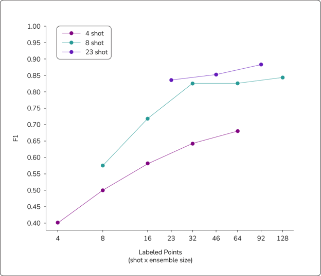
Figure 4: Results of experiments to judge the effectiveness of ensembling with varying shot counts. With lower shot counts, ensembling improved performance, but the 23-shot prompts still returned more accurate results.
We labeled the x-axis as the total number of labeled points for each strategy. For example, the rightmost blue point is 8-shot with an ensemble of size 16, which resulted in labeling a total of 128 points. The leftmost point of each shot count is an ensemble of size 1, which just means that we didn’t ensemble. The largest test we did of the 4- and 8-shots was an ensemble of 16, and the largest for 23-shot was an ensemble of four. It is important to note that the number of labeled points is not just indicative of labeling constraints. The larger shot counts also require more computation. For example, 23-shots with an ensemble of four was similar in total computation to an 8-shot with an ensemble of 16.
As we can see, with all three shot counts, performance improved significantly with ensemble size. The performance increase was the most significant for lower shot counts, perhaps due to the high variance with fewer shots. For example, a 4-shot ensemble of two is swayed much more by a poor or inaccurate result than a 4-shot ensemble of 16.
Despite the improvements, the lower shot counts did not surpass the performance of the 23-shot ensembles. The 23-shot ensembles still showed clear improvement with ensemble size, but a less significant one. These results suggest that ensembling is useful, but it still remains better to do a small ensemble with a high shot count than to do a large ensemble with a small shot count.
Conclusions About Unsupervised Learning Methods for Text Classification
Our experiments have shown strong potential for using unsupervised learning methods for text classification with LLMs—with a few caveats. The element that is most critical to getting good results with this approach is the use of shots: examples of the results you want the LLM to produce.
As shown through our tests, the more shots you can include in your prompt, the better. Notably, variations in those shots do not significantly alter the results. Using static, randomly selected examples performs only slightly worse than carefully selecting them through a k-nearest neighbors algorithm. Likewise, ensembling improves the F1 score of LLM text classification, but the prompts with more shots still perform much better than those with fewer—even when using large ensembles.
Ultimately, these experiments show that unsupervised learning can produce worthwhile text classification inferences. In our next post, we’ll look at how both supervised and unsupervised methods stack up and explore considerations for each approach when trying to classify text.
Want to know how you can perform text classification with Striveworks? Reach out to schedule a demo of our platform today.
References
- Reimers, Nils and Iryna Gurevych. “Sentence-BERT: Sentence Embeddings Using Siamese BERT-Networks.” *ArXiv preprint arXiv:1908.10084* (2019).
- Ratner, Nir, Yoav Levine, Yonatan Belinkov, Ori Ram, Inbal Magar, Omri Abend, Ehud Karpas, Amnon Shashua, Kevin Leyton-Brown, and Yoav Shoham. “Parallel Context Windows for Large Language Models.” *ArXiv preprint arXiv:2212.10947* (2022).
- Yang, Kejuan, Xiao Liu, Kaiwen Men, Aohan Zeng, Yuxiao Dong, and Jie Tang. “Revisiting Parallel Context Windows: A Frustratingly Simple Alternative and Chain-of-Thought Deterioration.” ArXiv abs/2305.15262 (2023).
